How to Build a Centralised Multi-Channel Report

Picture this. You are running digital marketing activity across LinkedIn, Facebook, and Google Ads for a single account. Each of these platforms has different objectives and budgets, but the client would like to have a centralized dashboard with visibility on all platforms in a table. In addition to this, the client uses Google Analytics as their single source of truth for business KPIs, and therefore need to be able to see conversions and leads (newsletter sign ups, transactions, revenue) imported from GA into said dashboard.

As a starting point, you are already extracting all the data to Google Sheets in order to create the new dashboard, using data extraction tools such as Funnel, Supermetrics and Adverity. However, each of these data sets sits in different tabs of your report, and now, you need to combine them.

To do so via Data Studio, despite being a comprehensive data visualisation tool, is simply impossible. Whilst Data Studio has left joints available, users are not able to “union the data” (stack tables on top of each other), which means that blending the data is therefore not an option.

So, how do we get all this data in a single table that can be used by Data Studio or other visualization tools?

A simple solution lies in the query functions of Google Sheet. These allow users to combine data from different tables into a single view, grouping data in any number of columns.

The function uses a syntax very similar to SQL, albeit with a few key differences. For instance, in SQL, to query a column, you would type in “Select ‘Column Name’”, whereas in Google Sheets query, the syntax is “Select ‘Column Range’” (ie, A, B, C…). Likewise, for a sum of column, you would do in SQL “Sum(Column Name)”, and in Google Sheets “Sum(Column Range)”.

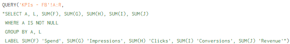
Example query on Google Sheets.

Selecting metrics and dimensions

A good first step is to think of all the columns needed for the final view. For example, does the client care about the performance of each individual campaign, or is grouping the performance of the campaigns against their desired objective enough? Or, are there groups of campaigns that are of interest within a single objective (retargeting vs prospecting on Facebook, or Generics vs Brand on Google)?

By applying a series of a VLookUps, you can assign objectives / groupings to all the campaigns (Pro tip – Use an arrayformula [=arrayformula(vlookup(‘lookup value range’…] to fill all the range with the formula, rather than pasting it manually).

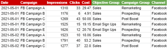
Example of data with Objectives to group rows by.

The next step is then to query all the data for the different sources into a single view. In order to query multiple tables on top of each other, you will need to use dynamic brackets ({}) and semicolons (;) (Pro tip – use Alt+Enter to create line breaks inside the formula for easier reading).

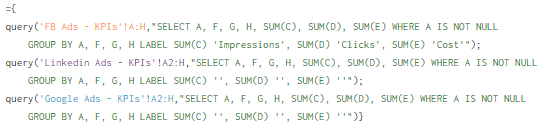
Example query combining data from three different tables.

In the above example query, you’ll see that the second and third query start from the second row (A2, as opposed to A). This is to avoid repetition of column titles through the data. This is also why the label function at the end of each query (“LABEL SUM(C) ‘ ‘”) has a blank in between the quotation marks, whereas Google Sheets would normally populate it with a “sum” cell as below:

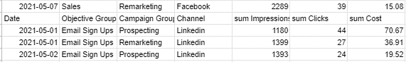
Result of querying full range instead of from row 2 in queries other than the first.

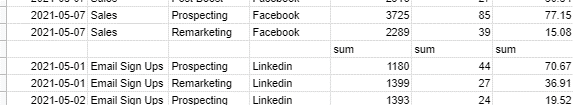
Result of not labelling calculated fields as ‘empty’ in queries other than the first.

Aligning the schemas

So, you have now merged your data from three different media sources into a single table, but we have yet to add in conversions. These are coming from Google Analytics, and whilst they can be segmented by data, source, and campaign, but they have no Impressions or cost associated with them (except for Google Ads data, if the Google Analytics and Google Ads accounts are linked).

A solution to merge data sets with missing KPIs is to create dummy columns with the missing KPIs populated with 0, so that they can be stacked to each other. This must be done on both on the merged media data, and the conversion data, adding in conversions onto the media KPIs, and media KPIs onto the conversion data. Again, you can use an arrayformula to populate the full range, but Google Sheets only requires the very first row to have values.

Conversion data added as 0 on the media KPIs table.

Media KPIs added as 0 on the conversion table.

Blending the data

From this step, you can now create a new query that combines the media KPIs and conversion data. But, be careful of the order in which each of the elements is called, as they must be called in the same order on both queries. Here is the query that merges the data from the two examples below:

Query merging media KPIs and analytics conversion data

And so there we have it, you now have a single table that combines data from multiple publishers, and conversion data from Analytics. This means that within a single dashboard you can accurately report on overall media CPA and ROAS, as well as report on CPA per campaign group, type, or channel!

On this link, you will also find dummy data from where these screenshots were taken:

https://docs.google.com/spreadsheets/d/18YELvW58d1PkDZ0olUlaUwCcbuoNz8JZh9qZCX8TR_Q/edit?usp=sharing 

Pierre Daudré-Vignier, Senior Account Manager